Load the R package we will use.

library(tidyverse)
library(moderndive) #install before loading

Quiz questions

Replace all the instances of ‘SEE QUIZ’. These are inputs from your moodle quiz.
Replace all the instances of ‘???’. These are answers on your moodle quiz.
Run all the individual code chunks to make sure the answers in this file correspond with your quiz answers
After you check all your code chunks run then you can knit it. It won’t knit until the

-??? are replaced

-The quiz assumes that you have watched the videos and worked through the examples in

Chapter 7 of ModernDive

Question:

7.2.4 in Modern Dive with different sample sizes and repetitions

Make sure you have installed and loaded the tidyverse and the moderndive packages
Fill in the blanks
Put the command you use in the Rchunks in your Rmd file for this quiz.

Modify the code for comparing different sample sizes from the virtual bowl

Segment 1: sample size = 28

1.a) Take 1150 samples of size of 28 instead of 1000 replicates of size 25 from the bowl dataset. Assign the output to virtual_samples_28

virtual_samples_28 <- bowl  %>% 
rep_sample_n(size = 28, reps = 1150)

1.b) Compute resulting 1150 replicates of proportion red

start with virtual_samples_28 THEN
group_by replicate THEN
create variable red equal to the sum of all the red balls
create variable prop_red equal to variable red / 28
Assign the output to virtual_prop_red_28

virtual_prop_red_28 <- virtual_samples_28 %>% 
  group_by(replicate) %>% 
  summarize(red = sum(color == "red")) %>% 
  mutate(prop_red = red / 28)

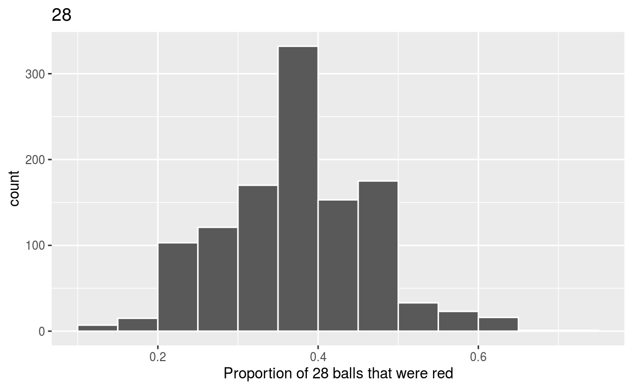
1.c) Plot distribution of virtual_prop_red_28 via a histogram

use labs to
label x axis = “Proportion of 28 balls that were red”
create title = “28”

ggplot(virtual_prop_red_28, aes(x = prop_red)) +
  geom_histogram(binwidth = 0.05, boundary = 0.4, color = "white") +
  labs(x = "Proportion of 28 balls that were red", title = "28")

Segment 2: sample size = 53

2.a) Take 1150 samples of size of 53 instead of 1000 replicates of size 50.

Assign the output to virtual_samples_53

virtual_samples_53 <- bowl  %>% 
rep_sample_n(size = 53, reps = 1150)

2.b) Compute resulting SEE QUIZ replicates of proportion red

start with virtual_samples_53 THEN
group_by replicate THEN
create variable red equal to the sum of all the red balls
create variable prop_red equal to variable red / 53
Assign the output to virtual_prop_red_53

virtual_prop_red_53 <- virtual_samples_53 %>% 
  group_by(replicate) %>% 
  summarize(red = sum(color == "red")) %>% 
  mutate(prop_red = red / 53)

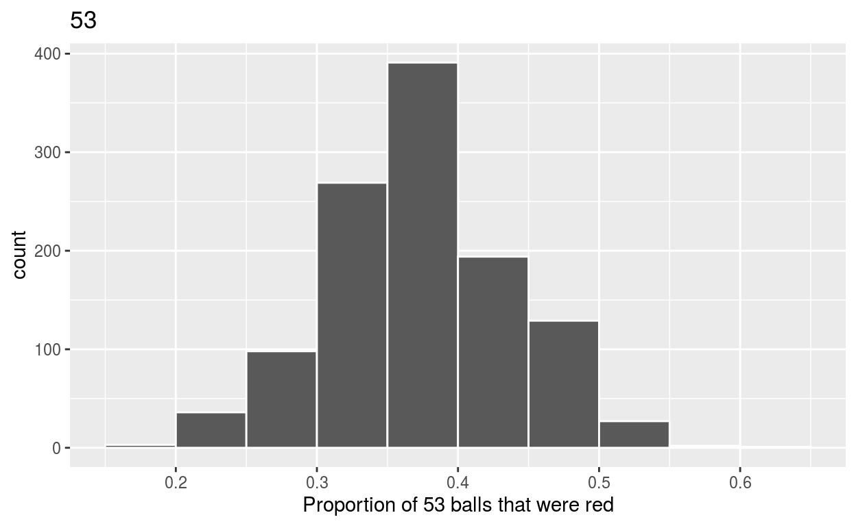
2.c) Plot distribution of virtual_prop_red_SEE QUIZ via a histogram

use labs to

label x axis = “Proportion of 53 balls that were red”
create title = “53”

ggplot(virtual_prop_red_53, aes(x = prop_red)) +
  geom_histogram(binwidth = 0.05, boundary = 0.4, color = "white") +
  labs(x = "Proportion of 53 balls that were red", title = "53")

Segment 3: sample size = 118

3.a) Take 1150 samples of size of 118 instead of 1000 replicates of size 50.

Assign the output to virtual_samples_118

virtual_samples_118  <- bowl  %>% 
rep_sample_n(size = 118, reps = 1150)

3.b) Compute resulting 1150 replicates of proportion red

start with virtual_samples_118 THEN
group_by replicate THEN
create variable red equal to the sum of all the red balls
create variable prop_red equal to variable red / 118
Assign the output to virtual_prop_red_118

virtual_prop_red_118 <- virtual_samples_118 %>% 
  group_by(replicate) %>% 
  summarize(red = sum(color == "red")) %>% 
  mutate(prop_red = red / 118)

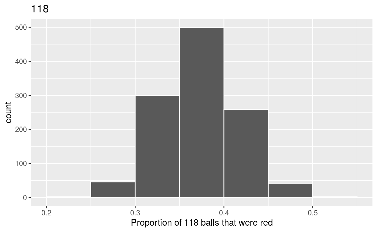
3.c) Plot distribution of virtual_prop_red_SEE QUIZ via a histogram

use labs to

label x axis = “Proportion of 118 balls that were red”
create title = “118”

ggplot(virtual_prop_red_118, aes(x = prop_red)) +
  geom_histogram(binwidth = 0.05, boundary = 0.4, color = "white") +
  labs(x = "Proportion of 118 balls that were red", title = "118")

Calculate the standard deviations for your three sets of SEE QUIZ values of prop_red using the standard deviation

n = 28

virtual_prop_red_28 %>% 
  summarize(sd = sd(prop_red))

# A tibble: 1 x 1
      sd
   <dbl>
1 0.0918

n = 53

virtual_prop_red_53 %>% 
  summarize(sd = sd(prop_red))

# A tibble: 1 x 1
      sd
   <dbl>
1 0.0663

n = 118

virtual_prop_red_118  %>% 
  summarize(sd = sd(prop_red))

# A tibble: 1 x 1
      sd
   <dbl>
1 0.0436

The distribution with sample size, n = 118 , has the smallest standard deviation (spread) around the estimated proportion of red balls.

Sampling

Question: